Chapter 5 Results

5.1 Representation of paricipants by different categories

First, let us check the representation of our participants. This answers the question if the sample of students participating in this research experiment is truly randomized. This can help us know if there is/are a group of people that is/are over-represented. In other words, it tells us about the selection bias.

We have chosen four characteristics of the participants: field of study, age, race, and intended career. Here are the bar plots for the same.

Note: The field, race, and career codes are summarized in the data key.

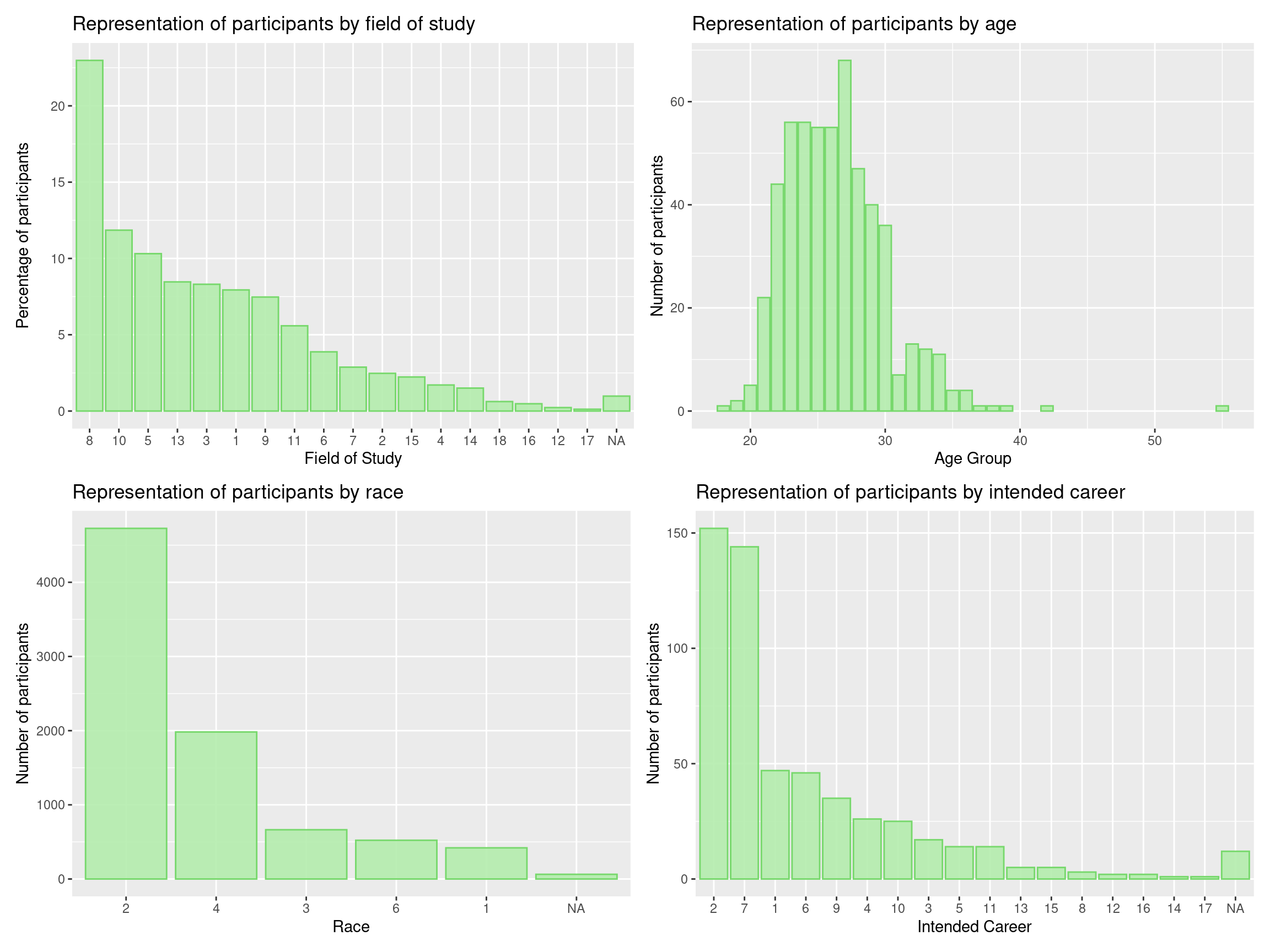
Here are the inferences from these plots:

1. For field of study

We can see that about 23% of the participants are from the 8th field of study, which is Business/Econ/Finance. This represents the highest percentage of students. Considering that this experiment was conducted by professors from the Columbia Business School, a lot of students from that field were expected. This is followed by fields 10 (Biological Sciences/Chemistry/Physics) and 5 (Engineering) representing the 2nd and 3rd highest percentages.

The 17th field of study, which is Architecture, constitutes about less than 1% of the participants. This is the least represented group in terms of field of study. Before that, comes field 12 (undecided), before which comes field 18 (other).

2. For age group

We can observe that most students are between the age 20 and 30, with about 68 people with age around 27. Almost all the participants are between 18 and 39 years of age, with the exception of a few of age 42 and 55.

3. For race

We can observe that race 2, which is European/Caucasian-American is the highest represented group here, which has about 4700 participants. Second most highest represented race is 4, i.e., Asian/Pacific Islander/Asian-American with about 2000 participants.

The count for race not specified is the least among all the races. Apart from that, the least represented race is Black/African American with about 450 participants.

4. For intended career

Here, we can observe that the intended career of most students is career 2 and 7, i.e., Academic/Research and Banking/Consulting/Finance/Marketing/Business/CEO/Entrepreneur/Admin respectively. They constitute for about 155 and 135 participants respectively. The least represented career field is career 17, which is Architecture. Similar trend was seen in the representation by field of study.

5.2 Number of yes matches per participant

In the original experiment, the variable match is the target variable. This indicates if the person was matched to the other person or not. We can use a Cleveland dot plot to show the number of yes matches each participant got. As mentioned before, we are using waves 10-21. Moreover, we faceted them by waves and color coded by the gender so we can also understand patterns among genders and within individual waves.

Here, we can observe that the maximum number of yes matches of participants in waves 10 and 13 is always less than 5. Also, the highest number of matches for waves 20 and 18 is 3. Waves 11, 14, 15, 18 and 21 have a wide variety of matches for different people.

Moreover, all waves have participants who are not matched with other people. The number of participants across all waves who did not get matched seem to have an even number of males and females. The most matched participant is a female from wave 21 who got 14 matches.

5.3 Analysing correlation between the chosen variables

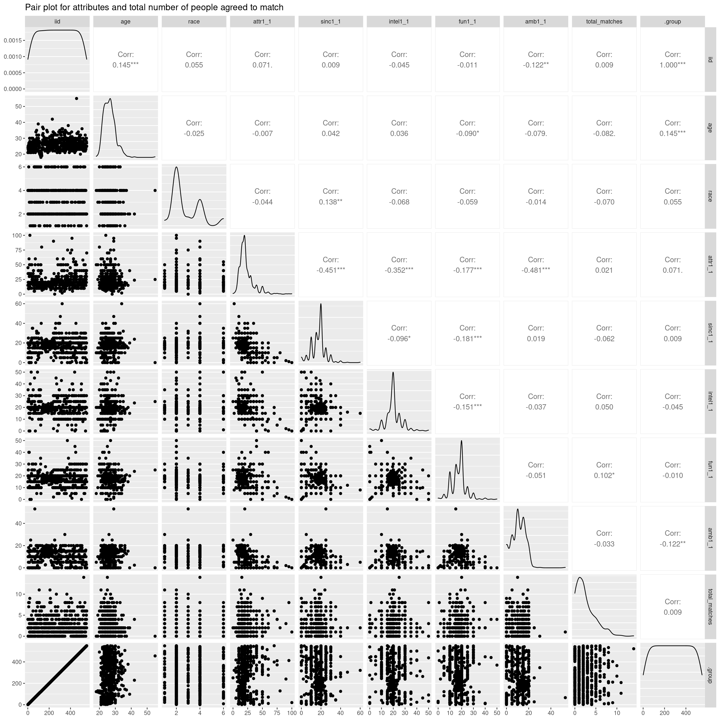
One of the important questions we want to address is visualizing whether the features in the dataset exhibit correlation among themselves or with the target variable that tells whether the pair matched or not. This is important as it will help us come up with blatant patterns observed in features that help in formulations of simple if-then rules. For the purposes of this visualization, we have narrowed down comparison of ratings to a specific question that were asked prior to the event - Distribute a score of 100 among the five attributes in the order of importance that you would like to see in your potential date.

This question is interesting to inspect if the attributes of what people look for in their potential partners bear any correlation among themselves and also with the actual number of people they agreed to match with.

Some of the interesting inferences we can make regarding the plots are,

The distribution of most of the attributes are close to normal except for ambition with seems to be right skewed. A relatively high number of participants have given a low priority to ambition of their potential partners as a deciding factor.
While most of the features are weakly negatively correlated almost exhibiting no correlation at all, the pair of feature sincerity, attractiveness and sincerity, intelligence are negatively correlated by the greatest amount. This tells us that people who gave a high preference to sincerity gave a low preference to intelligence and attractiveness and the other set of people weighed attractiveness and intelligence over sincerity.
The age of the participants are mostly between 20 and 30, while one senior participant over 50 did not match with anyone, evident by the anomaly of the farthest point in the age vs total_matches plot.
The trend that is seen in all the plots of attributes of attractiveness, sincerity, intelligence, fun and ambition is that, as the rating or the priority of certain feature increases, the number of matches goes down, for a few points. This is justifiable with the points that are to the farthest right at the bottom. This is expected as participants who have a really high expectation on one feature might not find someone suitable to meet their high expectations on that feature.
It is interesting to note that the same plot of features vs total matches also exhibits some anomaly. There seems to be one point in all these plots that have a relatively medium level rating/priority while the number of matches is pretty high. This can be verified by the top most point to the left of the plots. There were some participants who are estimated to have based their criteria of matching on factors others that the ones that were rated on. This can be infered as they have a relatively high number of matches than their peers who matched less, given the same priority for those features.

5.4 Analysis of decision making on Race

One of the factors of taken into consideration for understanding the requirements of participant’s expectation with their partners is the Race. Each participant is required to report a rating out of 10 for their potential partner to be of the same race as them. This visualization is to analyze whether the actual decision of the partcipants is influenced by any other factors that overpowers them to match with their dates from Race other than their own.

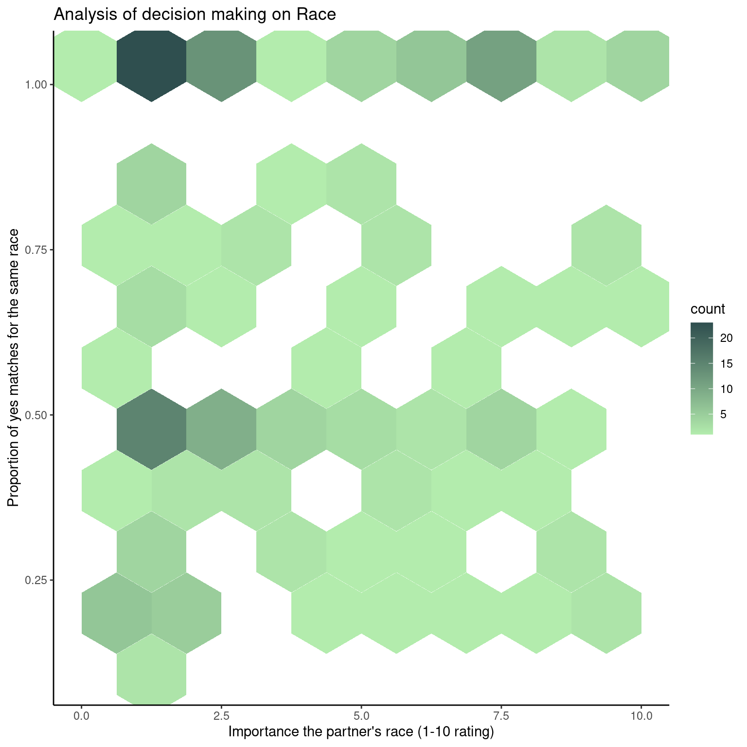
The following hexmap is a visual of Proportion of Matches that interested the participants from the same Race vs Importance of Race reported before the actual experiment.

The hexmap uncovers some interesting patterns observed from the participants’ responses,

There are instances of participants matching with only participants of different Races irrespective of their response to Importance of same Race. This indicates that Race is clearly not the sole factor for making a decision of matching with people.
There is one anomaly at the top right hex cell which has the highest count of people matching with participants of the same Race despite giving a lower priority on importance of same Race.
The count of people who have a high importance to matching with the same Race but indeed have agreed to match with the same Race are relatively low. This is indicated by light green hex patches implying a lower frequency of people matching within their own race.
The presence of hexagons on the lower proportion of matches within the same race for higher values of importance of Race is intriguing. From this we can infer that participants who were strongly inclined to match with their own Race, changed their mind after the experiment. This gives a clear indicator that other attributes of a person overpowered their mindset of same Race.

5.5 Attribute Rating Analysis by Race

From the previous plot we inferred that certain attributes are strong enough to change participant’s prior perception of importance of Race. Diving further, we want to understand how the attributes are rated for differently across the Race of the participants. This sheds light on how certain group of participants, characteristically from a certain Race, have prioritized attributes in their potential partners. Below is a mosaic plot for two specific features - attractiveness and ambition as independent features and visualized by Race as the dependent variable.

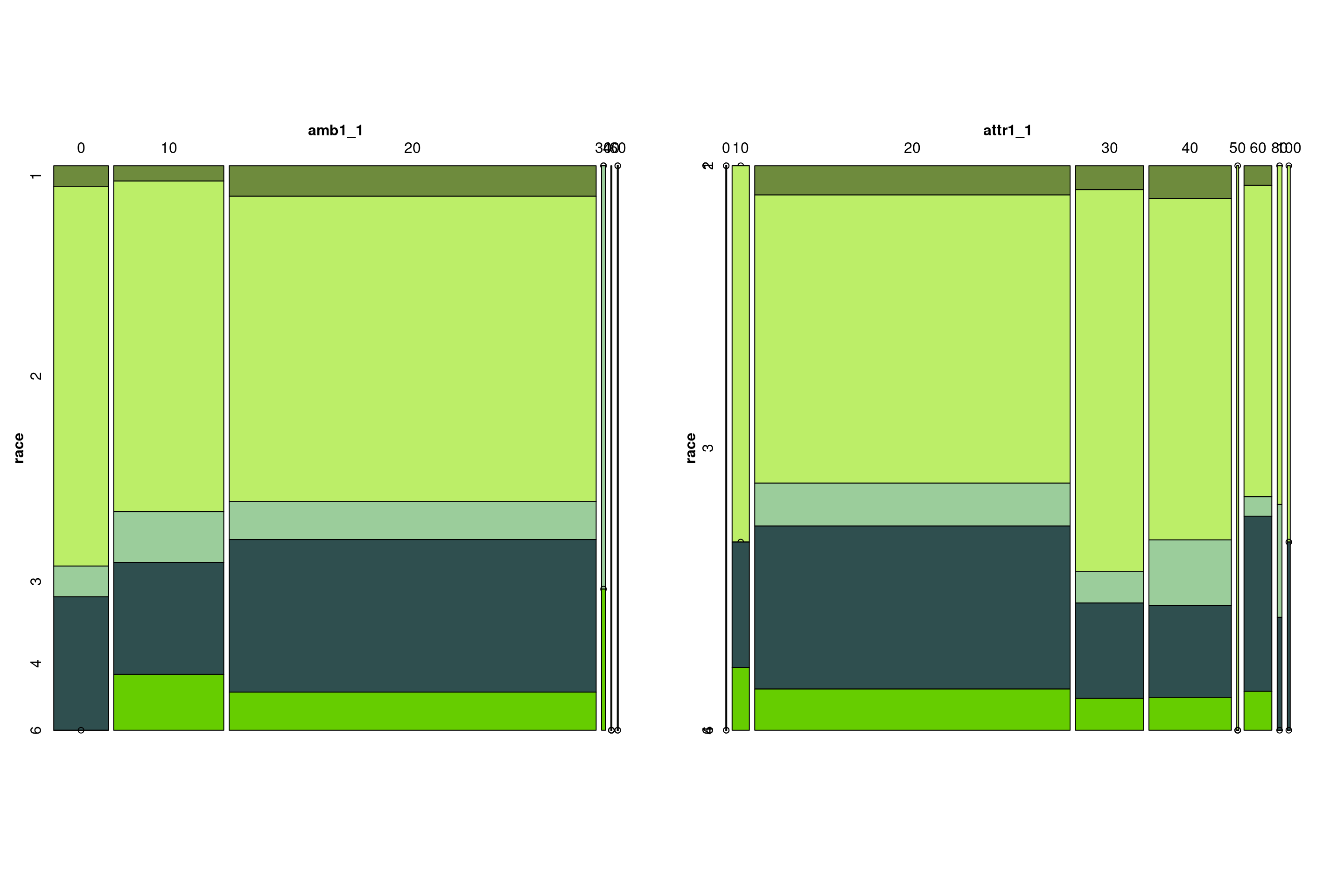
NOTE: The reason for not following a palette/gradient colour scheme for mosaic plots is to easily distinguish the depend variable for smaller count indicated by smaller rectangles to the right.

Some of the inferences we can draw from the above mosaic plots of attributes - attractiveness and ambition are,

Race 1 - Seems to have a nearly equal distribution across all the bins for attractiveness while only upto importance of 20 for ambition.
Race 2 and Race 4- Majority of the participants are from Race 2 followed by Race 4 and the distribution of importance for ambition is split from 0 to 20. While the distribution of ratings for attractiveness is spread across a range of 0-100. This is a clear indication that Race 2 and Race 4 values attractiveness over ambition and is likely to be comprised over the younger population who value attractiveness more than anything.
Race 3 - Apparently has a greater distribution spanning until rating of 30-40 for ambition for a smaller set of population while attractiveness is equally distributed throughout. We suspect that Race 3 could comprise of a small set of higher age groups that are mature enough to value ambitiion in addition to attractiveness.
Race 5 - Follows a trend reverse in the direction of ratings in relation to the others, i.e, Ambition and Attractiveness is valued with almost equal distribution spanning from 10 - 60. Although the higher values seem to have characteristically low sized rectangles, they are unique as there are instances where participants exist who find both these disparate attributes important. We can infer that they might either contain an good representation of male and female ratio or a good representation of the comprehensive age groups.

5.6 Change of feature perception with time

Here, our objective is to find that if a participant’s perspective (ratings) on which features they are looking for in the opposite sex change with time, especially before and after the speed dating experiment. For this part, we chose one question in particular from the survey:

What you look for in the opposite sex?

Now, this question was asked to the same people multiple times. We specifically choose three times. The times we chose were:

Asked before the speed dating experiment
Asked the day after the speed dating experiment
Asked 3-4 weeks after the speed dating experiment

To answer our question, we decided to use parallel coordinate axis plots since it helps us to visualize multiple variables at once and also account for correlations among the variables by comparing the direction of the lines (which are our participants in this case). We color coded them by gender to find more inferences. Again, we used waves 10-21 for this plot.

We did this for each of the five features: Attractiveness, Sincerity, Intelligence, Fun, and Ambition. We normalized the values of each variable in the plots using the uniminmax scale. We did not use splines because we believe we lost information if we include it.

Here are the plots:

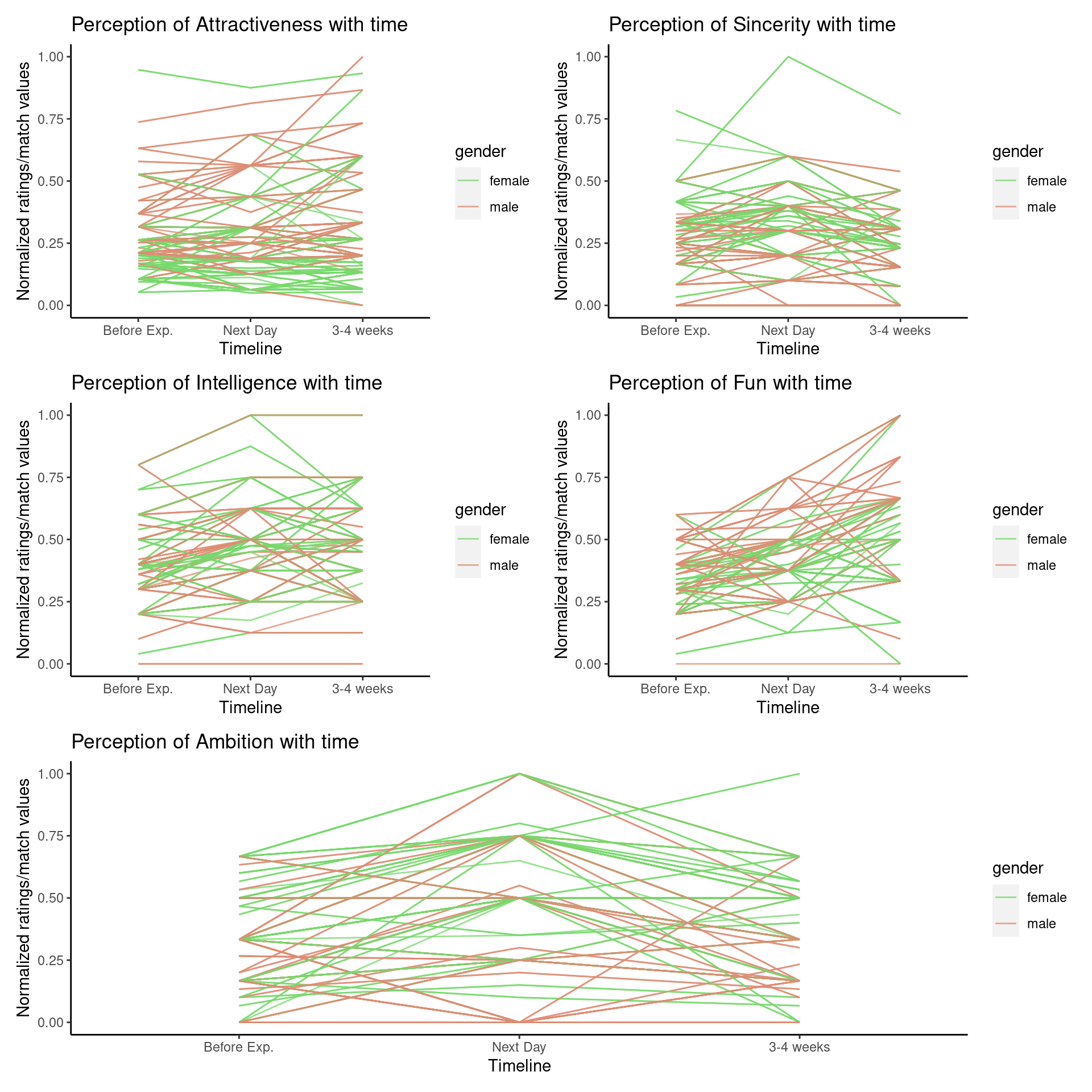
Here are the interpretations from the above plot:

1) For Attractiveness

Since most lines go slightly upwards from attr1_1 to attr1_2, we can say that people give slightly more importance to the attractiveness of the other person a day after the speed dating experiment. From attr1_2 to attr1_3, most lines go upward but some go downward. Hence, in general, most people give significant importance to the attractiveness of the partner. We can observe that few people drastically bring their rating from 25% to 100%, while some people reach 0% rating in 3-4 weeks. In general, the importance of attractiveness usually keeps increasing for males more, while there is no pattern for females. However, the increase of importance for females is more drastic in females.

2) For Sincerity

Since most lines go upwards from sinc1_1 to sinc1_2, we can say that people give more importance to the sincerity of the other person the next day. From sinc1_2 to sinc1_3, most lines go downward indicating that as most time passes (line 3-4 weeks), most people give less importance to the sincerity of the partner. For females, the importance of sincerity increases the day after the experiment, but reduces drastically in 3-4 weeks. For males, their sincerity importance level remained steady with time.

3) For Intelligence

Most lines go upwards from intel1_1 to intel1_2, some go downward, and some remain steady (especially the one with zero rating). Generally speaking, we can say that people give more intelligence to the sincerity right after the speed dating experiment. From intel1_2 to intel1_3, most lines remain steady, many go downward, and some go upward indicating that as most people remain around at similar levels or remain indifferent of their partner’s intelligence. For most males, the importance of intelligence increased after the experiment and remained steady afterward. For most females, it first increased too and then decreased.

4) For Fun

There does not seem to be a pattern from fun1_1 to fun1_2 or from fun1_2 to fun1_3 since many lines go upward and downward both times. Moreover, the variation in the range of ratings keep increasing from fun1_1 to fun1_3. Here too, the ratings of people with zero rating remained steady. No pattern is observed for particular genders.

5) For Ambition

Since most lines go upwards from amb1_1 to amb1_2, we can say that people give more importance to the ambition of the other person the next day. From amb1_2 to amb1_3, most lines go downward indicating that as most time passes (line 3-4 weeks), most people give less importance to the ambition of the partner. Here too, the ratings of people with zero rating remained steady. Moreover, some drastic increase (about 60% to 100%) and decrease (60% to 0%) of the importance of ambition is observed from amb1_1 to amb1_3. For females, the importance of ambition increased after the experiment, but decreased again in 3-4 weeks. For males, there seems to be an even distribution of people with increasing and decreasing importance.

5.7 Importance of attributes for each gender group

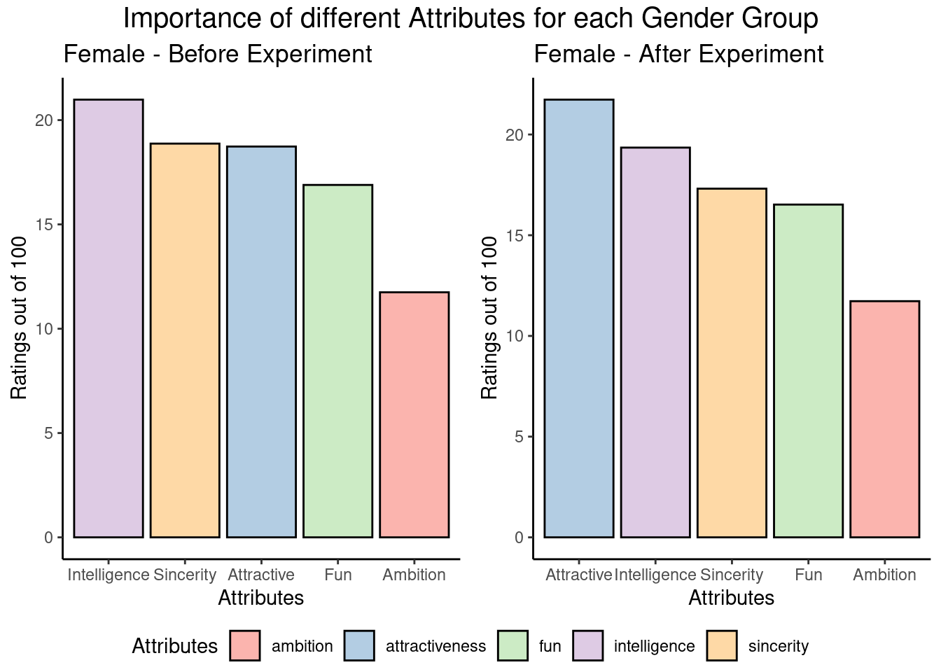
NOTE: The colours for the plots help in easy visualization of the order of the importance of attributes before and after the experiment.

It can be observed from the 1st plot that that most women before the Speed Dating Experiment rated Intelligence as most important attribute followed by Sincerity then Attractiveness. Whereas after the experiment women rated Attractiveness as the most important attribute followed by Intelligence then Sincerity.

It can be observed from the 2nd plot that most men before the Speed Dating Experiment rated Attractiveness as most important attribute followed by Intelligence then Fun. Even after the Experiment men rated Attractiveness as the most important attribute followed by Fun then Intelligence.

For both gender groups it can be observed that Ambition has been rated as the least important attribute. To female, the top three attributes are Intelligence, Sincerity and Attractiveness, while to male, they were Attractiveness, Intelligence and Fun. Also, it can be observed that men tended to have more distinctive preference whereas women’s preference appeared to be more even.

5.8 Comparison of Perception of Impotance of Attributes for each gender group

Before the Speed Dating experiment all the participants were asked to rate how important are these five attributes – Ambition, Attractiveness, Fun, Intelligence, Sincerity. They were asked to distribute 100 points across these attributes. They were also asked to rate what they think opposite sex would rate and what fellow women/men would rate how important the attributes are.

We get this information from the questions 1_1, 2_1, 4_1 for the data before experiment and 1_2, 2_2, 4_2 for the data after experiment. We plotted the average rating given by individual vs the rating given by opposite sex vs the rating of what fellow women/men would rate the attributes.

It can be observed from the plot that most women do not consider Attractiveness to be an important attribute but think that fellow women consider Attractiveness to be an important attribute. Similarly, even men think that women consider Attractiveness to be most important attribute but in real life women consider Intelligence to be the most important attribute.

It can be observed from the plot that men consider Attractiveness to be the most important attribute and also perceive that the fellow men also have same perception that Attractiveness is the most important attribute. It can also be observed that the women’s perception of what men think the most important attribute is correct as most women gave high rating for what men might rate for each attribute. We can also see that men don’t give much importance to their partner’s intelligence or ambition when it exceeds their own.

Overall, it can be observed that women’s perception of what men consider about each attribute is very accurate whereas men’s perception of what women might consider as important attributes is inaccurate (It can be seen in the difference between the pink bar and blue bar).

5.9 Satisfaction score vs. number of matches

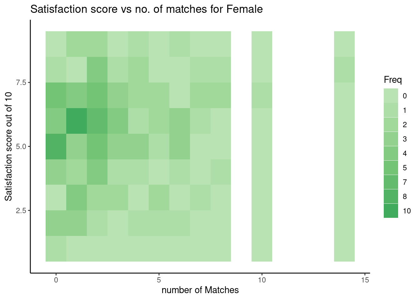
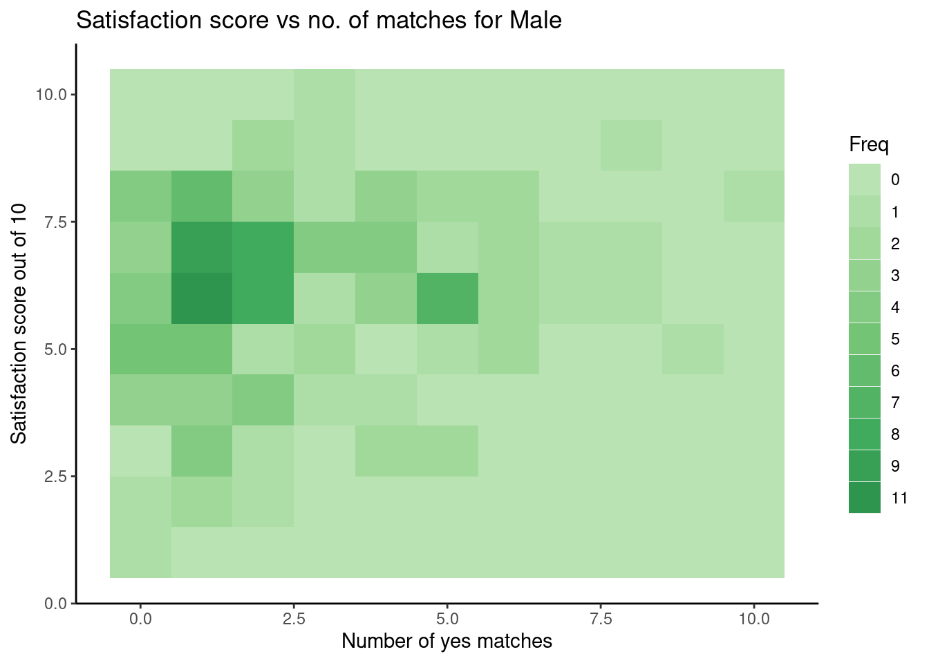
We plotted a heatmap to see the how the number of matches and the satisfaction score are distributed for the participants. The number of matches signifies the number of people they want to go on a 2nd date with and the satisfaction score signifies how satisfied they are with the experiment. We are calculating the frequency for the pairs of number of matches and satisfaction score. And plotting a heatmap to see what is the highest frequency pair.

From the first heatmap plotted for the females we can see that there are many people with 1 match and satisfaction score more than 5. Similar observations can be seen in the 2nd heatmap as well which is plotted for the males.

Overall, we can observe that people with lesser number of matches are more satisfied with the experiment. We can also infer than there are no females with 9, 11,12,13 number of matches. The data is left skewed as there are more people with 5 or lesser number of matches. Hence the plot is darker towards the left-hand side. We can also see that there are more people with satisfaction score of 5 or higher.

5.10 Actual Rating received vs Personal Perception vs Assumed Perception

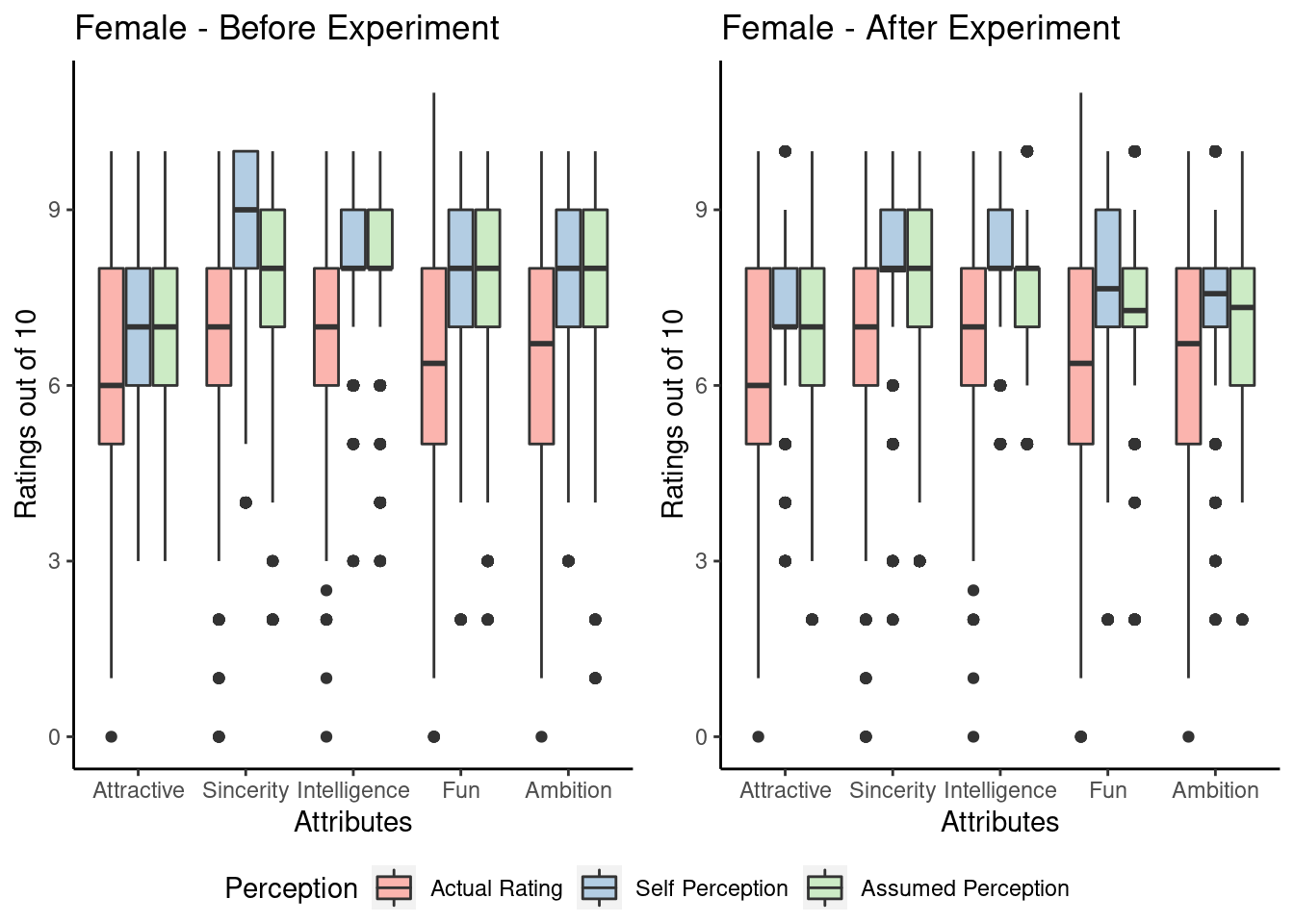
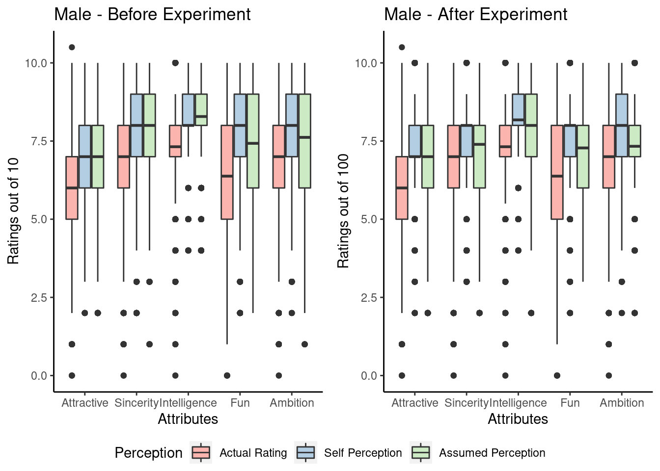
The participants were asked to rate themselves over the five attributes (Attractiveness, Sincerity, Intelligence, Fun and Ambition) on a scale of 1- 10 (1 being awful and 10 being great) they were also asked to rate their partners over these 5 attributes after each four-minute first date and were also asked how do they think others perceive them. The data for these questions is stored in questions 3_1, attr_o and 5_1 respectively. The participants were asked the same questions after the experiment as well the results for the questions are stored in 3_2 and 5_2 respectively.

We plotted box plots of the data to compare people’s actual rating vs self-perception vs what the participants assumed they would potentially receive. It can be observed while comparing self-ratings and the actual ratings, that the participants did generally overestimate themselves. The attribute that they overestimated the most was fun while the one that overestimated the least was intelligence. Females overestimated the attribute sincerity, most of the women rated themselves 9/10 where as most women received a score of 7/10. Whereas men overestimated the fun attribute most of the men rated themselves 8/10 but most received a score of 6.5/10.

It can also be seen from the results that most women increased their self-rating for the attributes after the experiment except from sincerity whereas most men decreased their self-rating for sincerity and fun. When comparing their assumed partner’s ratings and the actual ratings, we saw that while the participants knew that they were underestimated, the ratings they perceived were even lower than they thought over every attribute.